Go to this gist for original files.
1
2
3
4
5
6
7
8
9
10
11
12
13
14
15
16
17
18
19
20
21
22
23
24
25
26
27
28
29
30
31
| # -*- coding: utf-8 -*-
# @Author: MijazzChan, 2017326603075
# @ => https://mijazz.icu
# Python Version == 3.8
import os
import pandas as pd
import numpy as np
from matplotlib import pyplot as plt
import seaborn as sns
from sklearn.model_selection import train_test_split
from sklearn.metrics import accuracy_score
from sklearn.tree import DecisionTreeClassifier, export_text
from sklearn.utils import resample
from sklearn.metrics import confusion_matrix, classification_report
import warnings
%matplotlib inline
plt.rcParams['figure.dpi'] = 150
plt.rcParams['savefig.dpi'] = 150
sns.set(rc={"figure.dpi": 150, 'savefig.dpi': 150})
from jupyterthemes import jtplot
jtplot.style(theme='monokai', context='notebook', ticks=True, grid=False)
from IPython.core.display import HTML
HTML("""
<style>
.output_png {
display: table-cell;
text-align: center;
vertical-align: middle;
}
</style>
""");
|
Data Preprocessing
- Reading from
csv. - Replace
space( ) to underscore(_) in column names - check whether data containing nan/null.
- check if data gets any duplicated entries.
1
2
3
4
5
| original_data = pd.read_csv('./winequality-red.csv', encoding='utf-8')
# Tweaks header. GET RID OF THOSE DAMN SPACE!
new_columns = list(map(lambda col: str(col).replace(' ', '_'), original_data.columns.to_list()))
original_data.columns = new_columns
original_data.head(6)
|
| fixed_acidity | volatile_acidity | citric_acid | residual_sugar | chlorides | free_sulfur_dioxide | total_sulfur_dioxide | density | pH | sulphates | alcohol | quality |
|---|
| 0 | 7.4 | 0.70 | 0.00 | 1.9 | 0.076 | 11.0 | 34.0 | 0.9978 | 3.51 | 0.56 | 9.4 | 5 |
|---|
| 1 | 7.8 | 0.88 | 0.00 | 2.6 | 0.098 | 25.0 | 67.0 | 0.9968 | 3.20 | 0.68 | 9.8 | 5 |
|---|
| 2 | 7.8 | 0.76 | 0.04 | 2.3 | 0.092 | 15.0 | 54.0 | 0.9970 | 3.26 | 0.65 | 9.8 | 5 |
|---|
| 3 | 11.2 | 0.28 | 0.56 | 1.9 | 0.075 | 17.0 | 60.0 | 0.9980 | 3.16 | 0.58 | 9.8 | 6 |
|---|
| 4 | 7.4 | 0.66 | 0.00 | 1.8 | 0.075 | 13.0 | 40.0 | 0.9978 | 3.51 | 0.56 | 9.4 | 5 |
|---|
| 5 | 7.9 | 0.60 | 0.06 | 1.6 | 0.069 | 15.0 | 59.0 | 0.9964 | 3.30 | 0.46 | 9.4 | 5 |
|---|
1
2
| # Check whether data got null/na mixed inside.
original_data.isna().sum()
|
1
2
3
4
5
6
7
8
9
10
11
12
13
| fixed_acidity 0
volatile_acidity 0
citric_acid 0
residual_sugar 0
chlorides 0
free_sulfur_dioxide 0
total_sulfur_dioxide 0
density 0
pH 0
sulphates 0
alcohol 0
quality 0
dtype: int64
|
1
| original_data.describe().T
|
| count | mean | std | min | 25% | 50% | 75% | max |
|---|
| fixed_acidity | 1359.0 | 8.310596 | 1.736990 | 4.60000 | 7.1000 | 7.9000 | 9.20000 | 15.90000 |
|---|
| volatile_acidity | 1359.0 | 0.529478 | 0.183031 | 0.12000 | 0.3900 | 0.5200 | 0.64000 | 1.58000 |
|---|
| citric_acid | 1359.0 | 0.272333 | 0.195537 | 0.00000 | 0.0900 | 0.2600 | 0.43000 | 1.00000 |
|---|
| residual_sugar | 1359.0 | 2.523400 | 1.352314 | 0.90000 | 1.9000 | 2.2000 | 2.60000 | 15.50000 |
|---|
| chlorides | 1359.0 | 0.088124 | 0.049377 | 0.01200 | 0.0700 | 0.0790 | 0.09100 | 0.61100 |
|---|
| free_sulfur_dioxide | 1359.0 | 15.893304 | 10.447270 | 1.00000 | 7.0000 | 14.0000 | 21.00000 | 72.00000 |
|---|
| total_sulfur_dioxide | 1359.0 | 46.825975 | 33.408946 | 6.00000 | 22.0000 | 38.0000 | 63.00000 | 289.00000 |
|---|
| density | 1359.0 | 0.996709 | 0.001869 | 0.99007 | 0.9956 | 0.9967 | 0.99782 | 1.00369 |
|---|
| pH | 1359.0 | 3.309787 | 0.155036 | 2.74000 | 3.2100 | 3.3100 | 3.40000 | 4.01000 |
|---|
| sulphates | 1359.0 | 0.658705 | 0.170667 | 0.33000 | 0.5500 | 0.6200 | 0.73000 | 2.00000 |
|---|
| alcohol | 1359.0 | 10.432315 | 1.082065 | 8.40000 | 9.5000 | 10.2000 | 11.10000 | 14.90000 |
|---|
| quality | 1359.0 | 5.623252 | 0.823578 | 3.00000 | 5.0000 | 6.0000 | 6.00000 | 8.00000 |
|---|
1
2
3
4
5
6
7
8
9
10
11
12
13
14
15
16
17
18
19
| <class 'pandas.core.frame.DataFrame'>
RangeIndex: 1359 entries, 0 to 1358
Data columns (total 12 columns):
# Column Non-Null Count Dtype
--- ------ -------------- -----
0 fixed_acidity 1359 non-null float64
1 volatile_acidity 1359 non-null float64
2 citric_acid 1359 non-null float64
3 residual_sugar 1359 non-null float64
4 chlorides 1359 non-null float64
5 free_sulfur_dioxide 1359 non-null float64
6 total_sulfur_dioxide 1359 non-null float64
7 density 1359 non-null float64
8 pH 1359 non-null float64
9 sulphates 1359 non-null float64
10 alcohol 1359 non-null float64
11 quality 1359 non-null int64
dtypes: float64(11), int64(1)
memory usage: 127.5 KB
|
1
2
| # Look for duplicates
original_data.duplicated().sum()
|
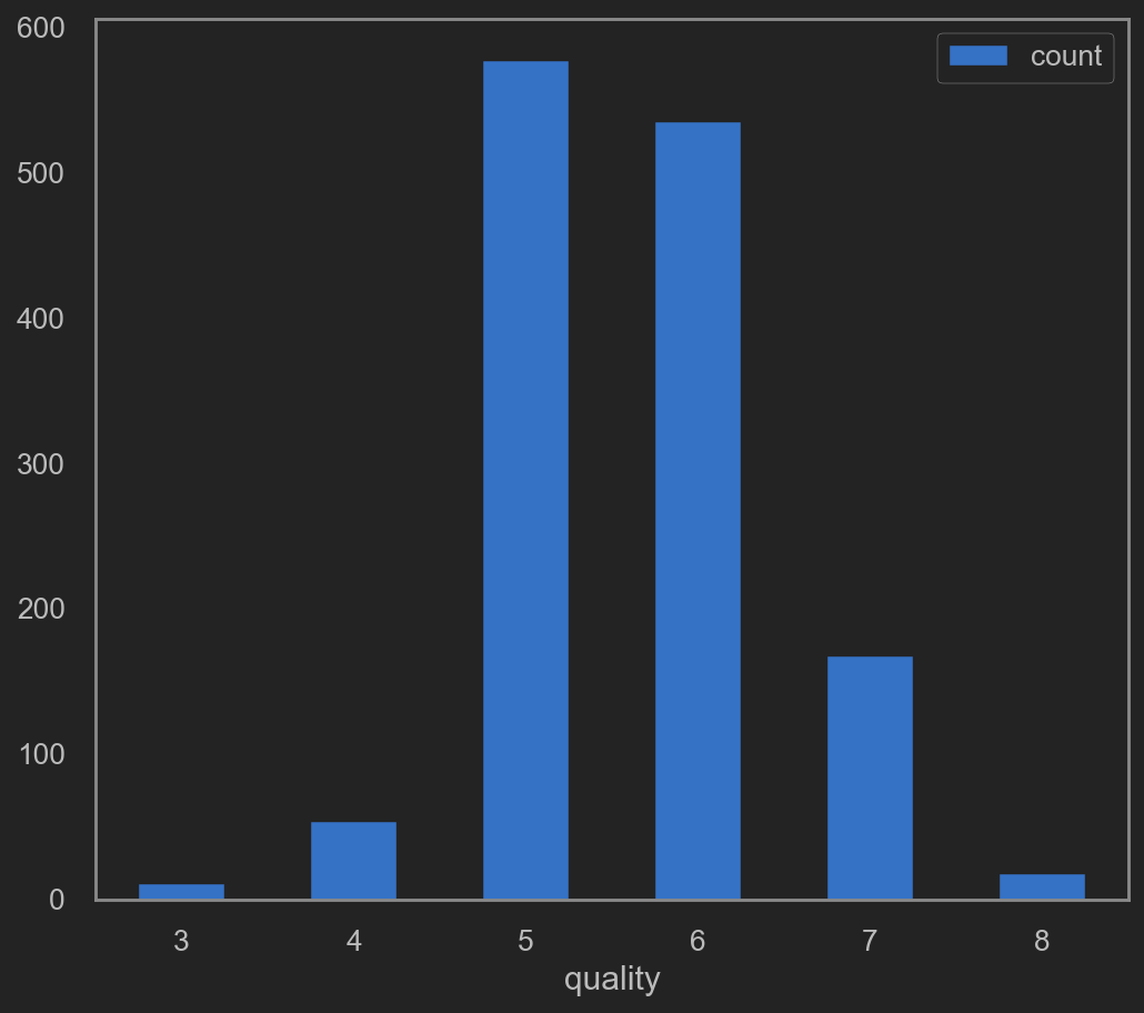
On quality(target) column
it seems that quality column only contains a few unique values. Go check that out shall we.
1
| original_data['quality'].unique().tolist()
|
1
2
3
4
| #original_data.groupby(['quality']).size().to_dict()
quality_plot_data = original_data.groupby(['quality']).size().reset_index()
quality_plot_data.columns = ['quality', 'count']
quality_plot_data.plot(kind='bar', x='quality', y='count', rot=0)
|
![png]()
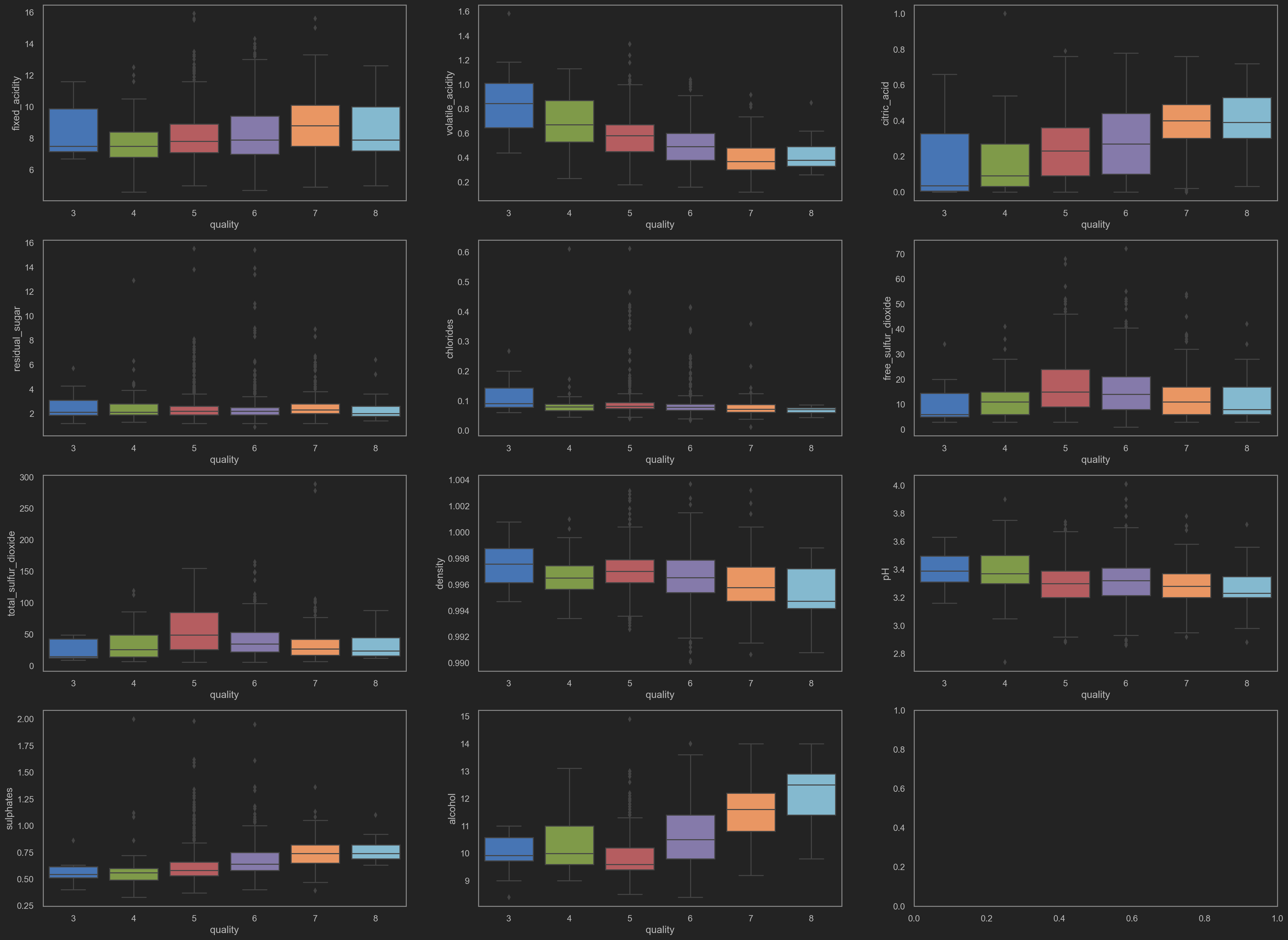
Data visualization
Box plots
Have a look at how each column data affects others.
1
2
3
4
5
6
7
8
9
10
11
12
13
| # tempX appended after each var is sort of a anti-corruption method? For me...
warnings.filterwarnings("ignore")
fig_temp1, ax_temp1 = plt.subplots(4, 3, figsize=(32, 24))
rolling_index = 0
columns_temp1 = list(original_data.columns)
columns_temp1.remove('quality')
for fig_row in range(4):
for fig_col in range(3):
sns.boxplot(x='quality', y=columns_temp1[rolling_index], data=original_data, ax=ax_temp1[fig_row][fig_col])
rolling_index += 1
if (rolling_index >= len(columns_temp1)):
break
plt.show()
|
![png]()
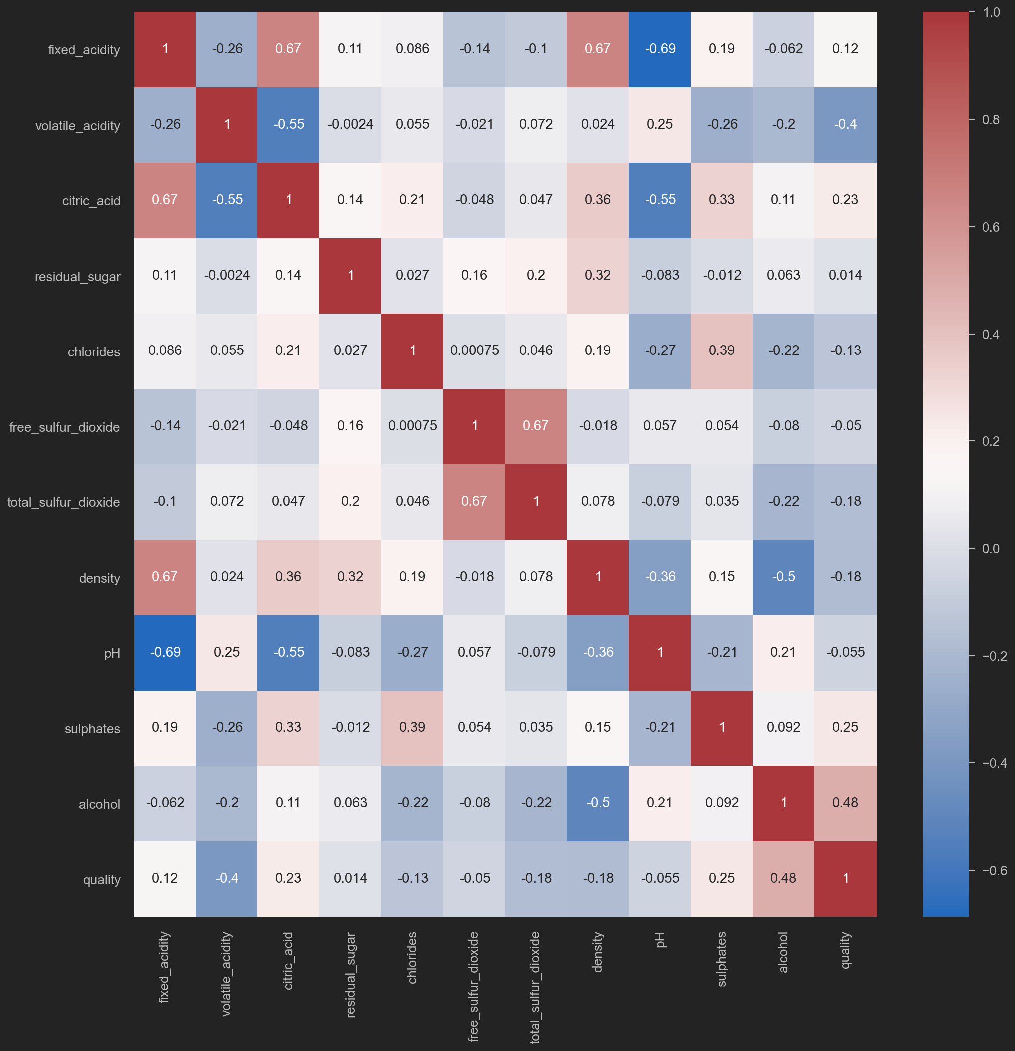
Heatmap on corr()
1
2
3
| # Need Square plot here temporaily
plt.figure(figsize=(16, 16))
sns.heatmap(original_data.corr(), annot=True, cmap='vlag')
|
![png]()
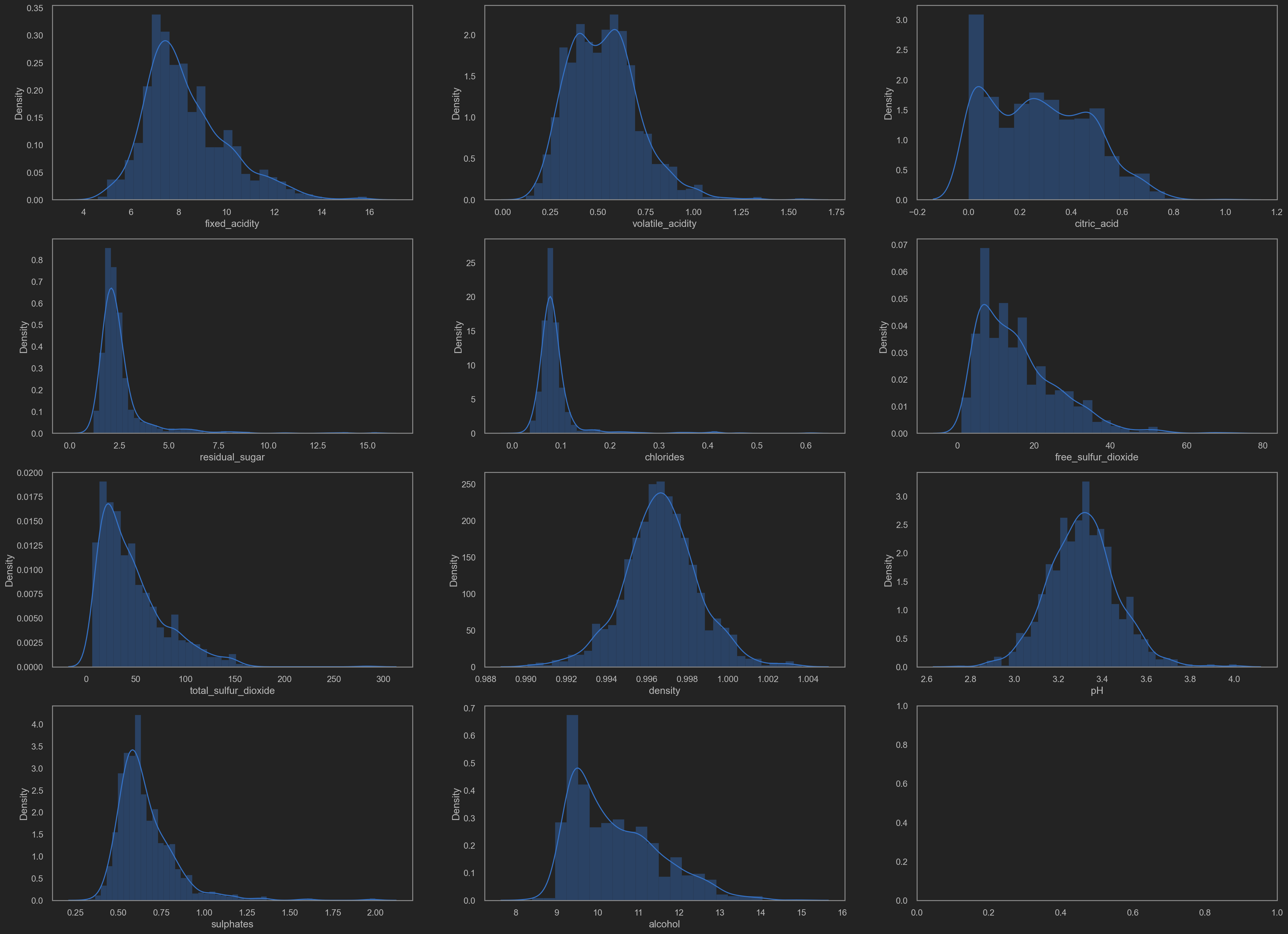
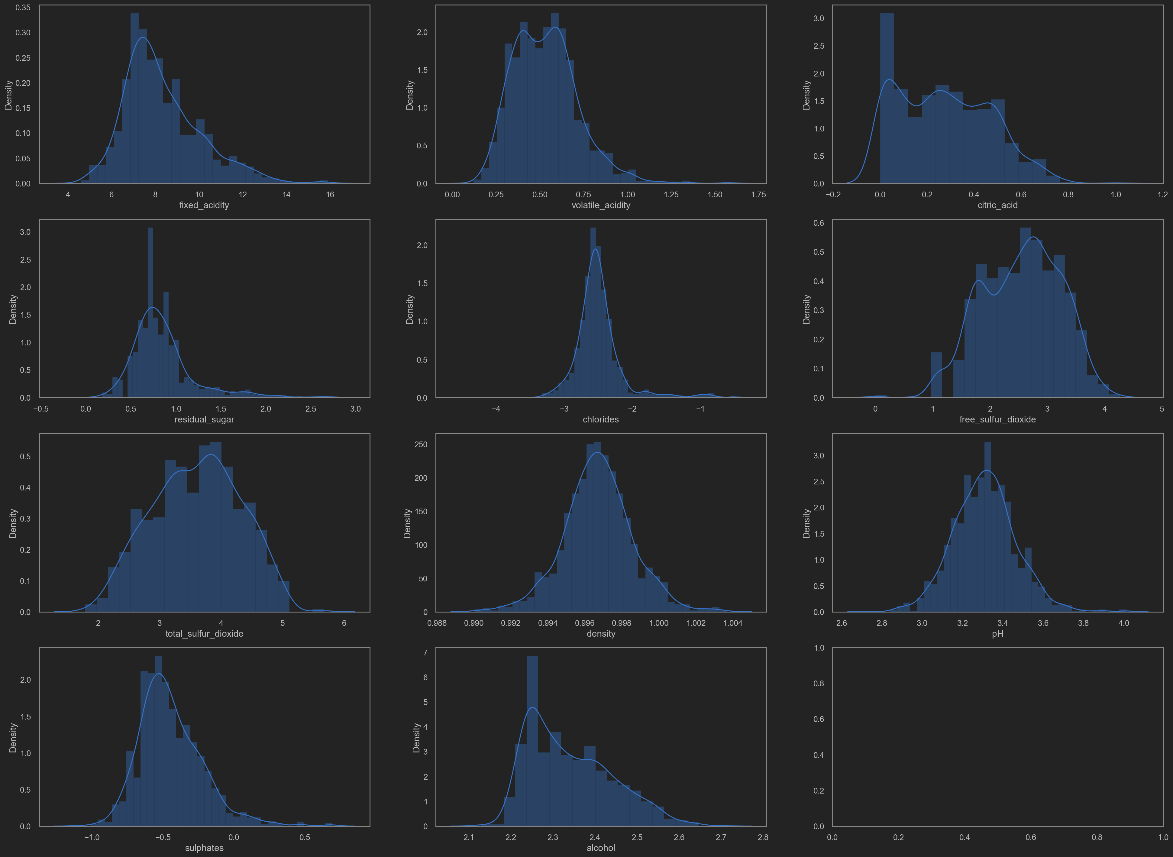
Distributions(distplot)
1
2
3
4
5
6
7
8
9
10
11
12
13
| # Anti-variable-corrupt kicks in.
warnings.filterwarnings("ignore")
fig_temp2, ax_temp2 = plt.subplots(4, 3, figsize=(32, 24))
rolling_index = 0
columns_temp2 = list(original_data.columns)
columns_temp2.remove('quality')
for fig_row in range(4):
for fig_col in range(3):
sns.distplot(original_data[columns_temp2[rolling_index]], ax=ax_temp2[fig_row][fig_col])
rolling_index += 1
if (rolling_index >= len(columns_temp2)):
break
|
![png]()
Minor tweaks based on the visualization plot
Why?
It is noticeable that some data distributing in a skew way. No good for training.
TODO: log trans? or sigmoid trans? MijazzChan @ 20210510220732
Let’s add some transformation shall we.
- residual sugar
- chlorides
- free SO2
- total SO2
- sulphates
- alcohol
1
2
3
4
5
6
7
8
| def trans_tweaks(col):
return np.log(col[0])
tweaked_data = original_data.copy()
cols_need_tweaks = ['residual_sugar', 'chlorides', 'free_sulfur_dioxide', 'total_sulfur_dioxide', 'sulphates', 'alcohol']
for each_col in cols_need_tweaks:
tweaked_data[each_col] = original_data[[each_col]].apply(trans_tweaks, axis=1)
# Tweaks completed.
|
Tweak result
distribution after transform.
1
2
3
4
5
6
7
8
9
10
| fig_temp3, ax_temp3 = plt.subplots(4, 3, figsize=(32, 24))
rolling_index = 0
columns_temp3 = list(tweaked_data.columns)
columns_temp3.remove('quality')
for fig_row in range(4):
for fig_col in range(3):
sns.distplot(tweaked_data[columns_temp3[rolling_index]], ax=ax_temp3[fig_row][fig_col])
rolling_index += 1
if (rolling_index >= len(columns_temp3)):
break
|
![png]()
Data Learning
Use sklearn build-in DecisionTree to make a approach.
1
2
3
4
5
6
7
| # use sklearn.model_selection.train_test_split to split train and test data.
X_temp1 = tweaked_data.drop(['quality'], axis=1)
Y_temp1 = tweaked_data['quality']
x_train, x_test, y_train, y_test = train_test_split(X_temp1, Y_temp1, random_state=99)
print(x_train.shape, x_test.shape, y_train.shape, y_test.shape)
print('which is {0} rows in training set, consisting of {1} features.'.format(x_train.shape[0], x_train.shape[1]))
print('Corespondingly, {} rows are included in testing set.'.format(x_test.shape[0]))
|
1
2
3
| (1019, 11) (340, 11) (1019,) (340,)
which is 1019 rows in training set, consisting of 11 features.
Corespondingly, 340 rows are included in testing set.
|
1
2
3
4
5
6
7
8
9
10
11
12
13
14
15
16
17
18
19
20
| # ID3 is entropy based DecisionTree.
entropy_decision_tree = DecisionTreeClassifier(criterion='entropy', max_depth=6)
# CART is gini based DecisionTree.
gini_decision_tree = DecisionTreeClassifier(criterion='gini', max_depth=6)
trees_apoch1 = [entropy_decision_tree, gini_decision_tree]
# Fit/Train
for tree in trees_apoch1:
tree.fit(x_train, y_train)
# Predict
entropy_predition = entropy_decision_tree.predict(x_test)
gini_predition = gini_decision_tree.predict(x_test)
# score
entropy_score = accuracy_score(y_test, entropy_predition)
gini_score = accuracy_score(y_test, gini_predition)
# print the damn result
print('ID3 - Entropy Decision Tree (prediction score) ==> {}%'.format(np.round(entropy_score*100, decimals=3)))
print('CART - Gini Decision Tree (prediction score) ==> {}%'.format(np.round(gini_score*100, decimals=3)))
|
1
2
| ID3 - Entropy Decision Tree (prediction score) ==> 58.235%
CART - Gini Decision Tree (prediction score) ==> 54.118%
|
1
2
3
4
5
6
7
8
9
| print(' ID3 - Entropy Decision Tree \n Confusion Matrix 或 判断矩阵 或 真假阴阳性矩阵 ==>\n{}'
.format(confusion_matrix(y_test, entropy_predition)))
print(' Classification Report 或 分类预测详细 ==>\n')
print(classification_report(y_test, entropy_predition))
print('*'*50 + '\n')
print(' CART - Gini Decision Tree \n Confusion Matrix 或 判断矩阵 或 真假阴阳性矩阵 ==> \n{}'
.format(confusion_matrix(y_test, gini_predition)))
print(' Classification Report 或 分类预测详细 ==>\n')
print(classification_report(y_test, gini_predition))
|
1
2
3
4
5
6
7
8
9
10
11
12
13
14
15
16
17
18
19
20
21
22
23
24
25
26
27
28
29
30
31
32
33
34
35
36
37
38
39
40
41
42
43
44
45
46
47
| ID3 - Entropy Decision Tree
Confusion Matrix 或 判断矩阵 或 真假阴阳性矩阵 ==>
[[ 0 1 2 0 0 0]
[ 0 3 8 0 0 0]
[ 0 0 109 28 2 0]
[ 0 3 56 67 7 0]
[ 0 1 10 22 19 0]
[ 0 0 0 1 1 0]]
Classification Report 或 分类预测详细 ==>
precision recall f1-score support
3 0.00 0.00 0.00 3
4 0.38 0.27 0.32 11
5 0.59 0.78 0.67 139
6 0.57 0.50 0.53 133
7 0.66 0.37 0.47 52
8 0.00 0.00 0.00 2
accuracy 0.58 340
macro avg 0.36 0.32 0.33 340
weighted avg 0.58 0.58 0.57 340
**************************************************
CART - Gini Decision Tree
Confusion Matrix 或 判断矩阵 或 真假阴阳性矩阵 ==>
[[ 0 0 3 0 0 0]
[ 1 0 7 3 0 0]
[ 0 0 94 42 3 0]
[ 0 0 48 74 10 1]
[ 0 0 8 28 16 0]
[ 0 0 0 1 1 0]]
Classification Report 或 分类预测详细 ==>
precision recall f1-score support
3 0.00 0.00 0.00 3
4 0.00 0.00 0.00 11
5 0.59 0.68 0.63 139
6 0.50 0.56 0.53 133
7 0.53 0.31 0.39 52
8 0.00 0.00 0.00 2
accuracy 0.54 340
macro avg 0.27 0.26 0.26 340
weighted avg 0.52 0.54 0.52 340
|
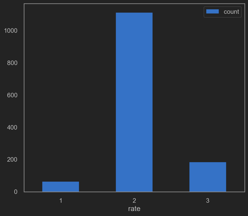
Train after grouped quality
It’s worth noticing that this prediction outcome falls into 6 zones.
Including quality in [3, 4, 5, 6, 7, 8].
Perhaps a little grouping may help.
DEFINE {quality == 3 or quality == 4} AS 1 (LOW quality)
DEFINE {quality == 5 or quality == 6} AS 2 (MID quality)
DEFINE {quality == 7 or quality == 8} AS 3 (HIGH quality)
Note that data prediction in this sector will only falls into [1, 2, 3] => [(3, 4), (5, 6), (7, 8)].
1
2
3
4
5
6
7
8
9
10
11
| def rate_transform(col):
if col[0] < 5:
return 1
elif col[0] < 7:
return 2
return 3
tweaked_data['rate'] = tweaked_data[['quality']].apply(rate_transform, axis=1)
rate_plot_data = tweaked_data.groupby(['rate']).size().reset_index()
rate_plot_data.columns = ['rate', 'count']
rate_plot_data.plot(kind='bar', x='rate', y='count', rot=0)
|
![png]()
This time, prediction will falls into 3 zones. As define above, RATE => [1, 2, 3] Try re-fit. This time, drop quality and rate. rate will be y.
1
2
3
4
5
6
7
8
9
10
11
12
13
14
15
16
17
18
19
20
21
22
| X_temp2 = tweaked_data.drop(['quality', 'rate'], axis=1)
Y_temp2 = tweaked_data['rate']
x_train, x_test, y_train, y_test = train_test_split(X_temp2, Y_temp2, random_state=99)
print(x_train.shape, x_test.shape, y_train.shape, y_test.shape)
print('which is {0} rows in training set, consisting of {1} features.'.format(x_train.shape[0], x_train.shape[1]))
print('Corespondingly, {} rows are included in testing set.\n'.format(x_test.shape[0]))
entropy_decision_tree = DecisionTreeClassifier(criterion='entropy', max_depth=5)
gini_decision_tree = DecisionTreeClassifier(criterion='gini', max_depth=5)
trees_apoch2 = [entropy_decision_tree, gini_decision_tree]
for tree in trees_apoch2:
tree.fit(x_train, y_train)
# Predict
entropy_predition = entropy_decision_tree.predict(x_test)
gini_predition = gini_decision_tree.predict(x_test)
# score
entropy_score = accuracy_score(y_test, entropy_predition)
gini_score = accuracy_score(y_test, gini_predition)
# print the result again.
print('ID3 - Entropy Decision Tree (prediction score) ==> {}%'.format(np.round(entropy_score*100, decimals=3)))
print('CART - Gini Decision Tree (prediction score) ==> {}%'.format(np.round(gini_score*100, decimals=3)))
|
1
2
3
4
5
6
| (1019, 11) (340, 11) (1019,) (340,)
which is 1019 rows in training set, consisting of 11 features.
Corespondingly, 340 rows are included in testing set.
ID3 - Entropy Decision Tree (prediction score) ==> 82.059%
CART - Gini Decision Tree (prediction score) ==> 78.824%
|
1
2
3
4
5
6
7
8
9
| print(' ID3 - Entropy Decision Tree \n Confusion Matrix 或 判断矩阵 或 真假阴阳性矩阵 ==>\n{}'
.format(confusion_matrix(y_test, entropy_predition)))
print(' Classification Report 或 分类预测详细 ==>\n')
print(classification_report(y_test, entropy_predition))
print('*'*50 + '\n')
print(' CART - Gini Decision Tree \n Confusion Matrix 或 判断矩阵 或 真假阴阳性矩阵 ==> \n{}'
.format(confusion_matrix(y_test, gini_predition)))
print(' Classification Report 或 分类预测详细 ==>\n')
print(classification_report(y_test, gini_predition))
|
1
2
3
4
5
6
7
8
9
10
11
12
13
14
15
16
17
18
19
20
21
22
23
24
25
26
27
28
29
30
31
32
33
34
35
| ID3 - Entropy Decision Tree
Confusion Matrix 或 判断矩阵 或 真假阴阳性矩阵 ==>
[[ 0 14 0]
[ 1 260 11]
[ 0 35 19]]
Classification Report 或 分类预测详细 ==>
precision recall f1-score support
1 0.00 0.00 0.00 14
2 0.84 0.96 0.90 272
3 0.63 0.35 0.45 54
accuracy 0.82 340
macro avg 0.49 0.44 0.45 340
weighted avg 0.77 0.82 0.79 340
**************************************************
CART - Gini Decision Tree
Confusion Matrix 或 判断矩阵 或 真假阴阳性矩阵 ==>
[[ 2 12 0]
[ 3 250 19]
[ 0 38 16]]
Classification Report 或 分类预测详细 ==>
precision recall f1-score support
1 0.40 0.14 0.21 14
2 0.83 0.92 0.87 272
3 0.46 0.30 0.36 54
accuracy 0.79 340
macro avg 0.56 0.45 0.48 340
weighted avg 0.76 0.79 0.77 340
|
Learning on tweaked data
How to resample
Y-data seems a little bit inbalanced? Okay then, add some resample might work.
Going back to quality column, which contains 6 different values.
Hence drop the rate column we added before.
1
2
3
4
5
6
7
8
9
10
11
12
| # Drop the rate data we added before.
tweaked_data.drop(['rate'], inplace=True, axis=1)
df_3 = tweaked_data[tweaked_data['quality'] == 3]
df_4 = tweaked_data[tweaked_data['quality'] == 4]
df_5 = tweaked_data[tweaked_data['quality'] == 5]
df_6 = tweaked_data[tweaked_data['quality'] == 6]
df_7 = tweaked_data[tweaked_data['quality'] == 7]
df_8 = tweaked_data[tweaked_data['quality'] == 8]
i = 3
for each_df in [df_3, df_4, df_5, df_6, df_7, df_8]:
print('quality == {0} has {1} entries'.format(i, each_df.shape[0]))
i += 1
|
1
2
3
4
5
6
| quality == 3 has 10 entries
quality == 4 has 53 entries
quality == 5 has 577 entries
quality == 6 has 535 entries
quality == 7 has 167 entries
quality == 8 has 17 entries
|
It’s quite obvious that 3, 4, 7, 8 are minorities. 5, 6 are majorities.
Hence we up-sample 3, 4, 6, 7, 8 to 550 entries. down-sample 5 to 550 entries
1
2
3
4
5
6
| df_3_upsampled = resample(df_3, replace=True, n_samples=550, random_state=9)
df_4_upsampled = resample(df_4, replace=True, n_samples=550, random_state=9)
df_7_upsampled = resample(df_7, replace=True, n_samples=550, random_state=9)
df_8_upsampled = resample(df_8, replace=True, n_samples=550, random_state=9)
df_5_downsampled = df_5.sample(n=550).reset_index(drop=True)
df_6_upsampled = resample(df_6, replace=True, n_samples=550, random_state=9)
|
After Re-sample(upsample & downsample). Value count looks like this.
1
2
3
4
5
6
| resampled_dfs = [df_3_upsampled, df_4_upsampled, df_5_downsampled, df_6_upsampled, df_7_upsampled, df_8_upsampled]
resampled_data = pd.concat(resampled_dfs, axis=0)
i = 3
for each_df in resampled_dfs:
print('quality == {0} has {1} entries'.format(i, each_df.shape[0]))
i += 1
|
1
2
3
4
5
6
| quality == 3 has 550 entries
quality == 4 has 550 entries
quality == 5 has 550 entries
quality == 6 has 550 entries
quality == 7 has 550 entries
quality == 8 has 550 entries
|
Before data is sent to training. Minor tweak is advised here.
TODO: pre-train data process. MijazzChan@20210511-010817 TODO-FINISH: MijazzChan@20210511-032652
Try drop some unrelated columns/features?
1
| resampled_data.corr()['quality']
|
1
2
3
4
5
6
7
8
9
10
11
12
13
| fixed_acidity 0.125105
volatile_acidity -0.600034
citric_acid 0.384477
residual_sugar 0.009648
chlorides -0.377277
free_sulfur_dioxide 0.081144
total_sulfur_dioxide 0.057946
density -0.321477
pH -0.267204
sulphates 0.490420
alcohol 0.597137
quality 1.000000
Name: quality, dtype: float64
|
little note here:
corr() values is 皮尔逊积矩相关系数 或correlation coefficient. It stays within [-1, 1].
abs(corr()) 越逼近1, 即相关度越高.
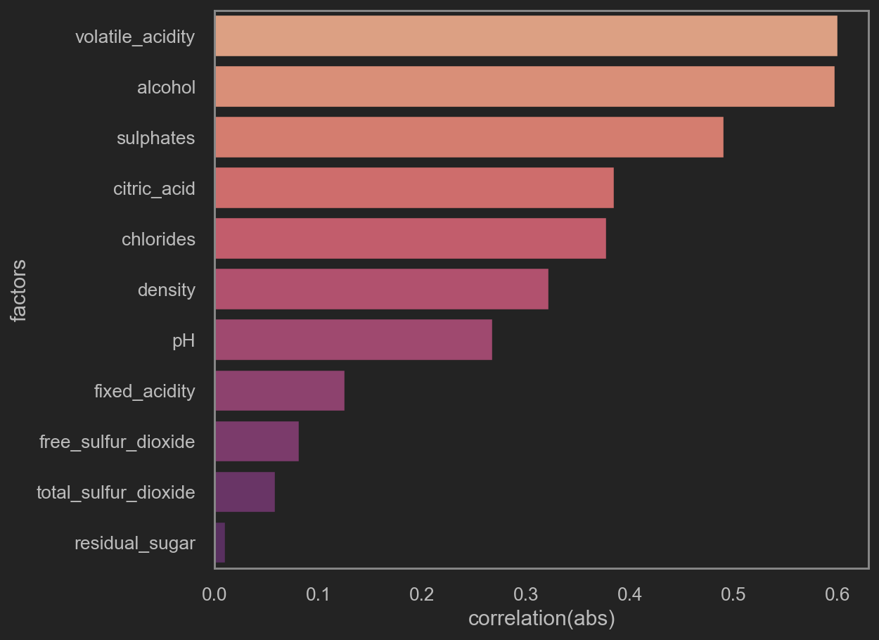
取abs后, 再看这些因素与quality的相关性.
After mapping with abs, we can review how much these columns are co-related with quality.
1
2
3
4
5
6
7
8
9
10
11
12
13
14
15
| def map_abs(col):
return np.abs(col[0])
corr_df = resampled_data.corr()['quality'].reset_index()
corr_df.columns = ['factors', 'correlation']
# quality is always related to quality, which means quality.corr == 1
# Hence the drop.
corr_df = corr_df[corr_df['factors'] != 'quality']
# Mapping with abs function
corr_df['correlation(abs)'] = corr_df[['correlation']].apply(map_abs, axis=1)
corr_df.sort_values(by='correlation(abs)', ascending=False, inplace=True)
corr_df.drop(['correlation'], inplace=True, axis=1)
print('TOP 5 quality-related factors\n', corr_df.head(5))
sns.barplot(x='correlation(abs)', y='factors', data=corr_df, orient='h', palette='flare')
|
1
2
3
4
5
6
7
| TOP 5 quality-related factors
factors correlation(abs)
1 volatile_acidity 0.600034
10 alcohol 0.597137
9 sulphates 0.490420
2 citric_acid 0.384477
4 chlorides 0.377277
|
![png]()
Note that only following factors is worth putting into training. They are
- volatile acidity
- alcohol
- sulphates
- citric acid
- chlorides
- density
- pH
- free sulfur dioxide
- fixed acidity
- total sulfur dioxide
Dropping factors as follows:
1
2
3
4
| factors_to_drop = ['residual_sugar']
simplified_data = resampled_data[resampled_data.columns[~resampled_data.columns.isin(factors_to_drop)]]
simplified_data.head(6)
|
| fixed_acidity | volatile_acidity | citric_acid | chlorides | free_sulfur_dioxide | total_sulfur_dioxide | density | pH | sulphates | alcohol | quality |
|---|
| 1106 | 7.6 | 1.580 | 0.00 | -1.987774 | 1.609438 | 2.197225 | 0.99476 | 3.50 | -0.916291 | 2.388763 | 3 |
|---|
| 1165 | 6.8 | 0.815 | 0.00 | -1.320507 | 2.772589 | 3.367296 | 0.99471 | 3.32 | -0.673345 | 2.282382 | 3 |
|---|
| 1253 | 7.1 | 0.875 | 0.05 | -2.501036 | 1.098612 | 2.639057 | 0.99808 | 3.40 | -0.653926 | 2.322388 | 3 |
|---|
| 1165 | 6.8 | 0.815 | 0.00 | -1.320507 | 2.772589 | 3.367296 | 0.99471 | 3.32 | -0.673345 | 2.282382 | 3 |
|---|
| 450 | 10.4 | 0.610 | 0.49 | -1.609438 | 1.609438 | 2.772589 | 0.99940 | 3.16 | -0.462035 | 2.128232 | 3 |
|---|
| 1165 | 6.8 | 0.815 | 0.00 | -1.320507 | 2.772589 | 3.367296 | 0.99471 | 3.32 | -0.673345 | 2.282382 | 3 |
|---|
Put the simplified df into training. See how it performs.
1
2
3
4
5
6
7
8
9
10
11
12
13
14
15
16
17
18
19
20
21
22
23
24
25
26
27
28
29
30
31
| X_temp3 = simplified_data.drop(['quality'], axis=1)
Y_temp3 = simplified_data['quality']
x_train, x_test, y_train, y_test = train_test_split(X_temp3, Y_temp3, random_state=99, test_size=0.3)
# Note that you don't use resampled data to test!!!!!!
# Drop duplicated row you added when resample.
# test_df = pd.concat([x_test, y_test], axis=1)
# print('test data containing duplicated entries(added during resample) => {}, drop them.'.format(test_df.duplicated().sum()))
# test_df.drop_duplicates(inplace=True)
# x_test = test_df.drop(['quality'], axis=1)
# y_test = test_df['quality']
print(x_train.shape, x_test.shape, y_train.shape, y_test.shape)
print('which is {0} rows in training set, consisting of {1} features.'.format(x_train.shape[0], x_train.shape[1]))
print('Corespondingly, {} rows are included in testing set.\n'.format(x_test.shape[0]))
entropy_decision_tree = DecisionTreeClassifier(criterion='entropy', splitter='random')
gini_decision_tree = DecisionTreeClassifier(criterion='gini', splitter='random')
trees_apoch3 = [entropy_decision_tree, gini_decision_tree]
for tree in trees_apoch3:
tree.fit(x_train, y_train)
# Predict
entropy_predition = entropy_decision_tree.predict(x_test)
gini_predition = gini_decision_tree.predict(x_test)
# score
entropy_score = accuracy_score(y_test, entropy_predition)
gini_score = accuracy_score(y_test, gini_predition)
# print the result.
print('ID3 - Entropy Decision Tree (prediction score) ==> {}%'.format(np.round(entropy_score*100, decimals=3)))
print('CART - Gini Decision Tree (prediction score) ==> {}%'.format(np.round(gini_score*100, decimals=3)))
|
1
2
3
4
5
6
| (2310, 10) (990, 10) (2310,) (990,)
which is 2310 rows in training set, consisting of 10 features.
Corespondingly, 990 rows are included in testing set.
ID3 - Entropy Decision Tree (prediction score) ==> 89.293%
CART - Gini Decision Tree (prediction score) ==> 89.697%
|
1
2
3
4
5
6
7
8
9
| print(' ID3 - Entropy Decision Tree \n Confusion Matrix 或 判断矩阵 或 真假阴阳性矩阵 ==>\n{}'
.format(confusion_matrix(y_test, entropy_predition)))
print(' Classification Report 或 分类预测详细 ==>\n')
print(classification_report(y_test, entropy_predition))
print('*'*50 + '\n')
print(' CART - Gini Decision Tree \n Confusion Matrix 或 判断矩阵 或 真假阴阳性矩阵 ==> \n{}'
.format(confusion_matrix(y_test, gini_predition)))
print(' Classification Report 或 分类预测详细 ==>\n')
print(classification_report(y_test, gini_predition))
|
1
2
3
4
5
6
7
8
9
10
11
12
13
14
15
16
17
18
19
20
21
22
23
24
25
26
27
28
29
30
31
32
33
34
35
36
37
38
39
40
41
42
43
44
45
46
47
| ID3 - Entropy Decision Tree
Confusion Matrix 或 判断矩阵 或 真假阴阳性矩阵 ==>
[[180 0 0 0 0 0]
[ 0 172 0 0 0 0]
[ 0 10 88 32 9 0]
[ 0 5 31 119 9 2]
[ 0 0 3 3 149 2]
[ 0 0 0 0 0 176]]
Classification Report 或 分类预测详细 ==>
precision recall f1-score support
3 1.00 1.00 1.00 180
4 0.92 1.00 0.96 172
5 0.72 0.63 0.67 139
6 0.77 0.72 0.74 166
7 0.89 0.95 0.92 157
8 0.98 1.00 0.99 176
accuracy 0.89 990
macro avg 0.88 0.88 0.88 990
weighted avg 0.89 0.89 0.89 990
**************************************************
CART - Gini Decision Tree
Confusion Matrix 或 判断矩阵 或 真假阴阳性矩阵 ==>
[[180 0 0 0 0 0]
[ 0 172 0 0 0 0]
[ 3 10 84 31 9 2]
[ 0 4 22 125 11 4]
[ 0 0 0 4 151 2]
[ 0 0 0 0 0 176]]
Classification Report 或 分类预测详细 ==>
precision recall f1-score support
3 0.98 1.00 0.99 180
4 0.92 1.00 0.96 172
5 0.79 0.60 0.69 139
6 0.78 0.75 0.77 166
7 0.88 0.96 0.92 157
8 0.96 1.00 0.98 176
accuracy 0.90 990
macro avg 0.89 0.89 0.88 990
weighted avg 0.89 0.90 0.89 990
|
The outcome is quite satisfying given that the predition this time falls into 6 zones.
这次预测的结果已经比较让人满意了, 因为预测值并非像先前加入rate一样, 只预测3个结果(LOW MID HIGH). 本次的预测结果是直接落入准确的[3,4,5,6,7,8]里的.
make a simple text visualization on the DecisionTree
1
| print(export_text(entropy_decision_tree, feature_names=x_train.columns.to_list()))
|
1
2
3
| Content too long to display.
# Goto Gist for original file:
# https://gist.github.com/MijazzChan/00f39ed1f17e6026ab3b1be94fc8e636
|